Content from Using RMarkdown
Last updated on 2025-11-11 | Edit this page
Overview
Questions
- How do you write a lesson using R Markdown and sandpaper?
Objectives
- Explain how to use markdown with the new lesson template
- Demonstrate how to include pieces of code, figures, and nested challenge blocks
Introduction
This is lesson, created follwing The Carpentries Workbench, is meant to be an introduction to learning how to work with timeseries datasets in R.
There are three sections that will appear at the start of every lesson:
-
questionsare displayed at the beginning of the episode to prime the learner for the content. -
objectivesare the learning objectives for an episode displayed with the questions. -
keypointsare displayed at the end of the episode to reinforce the objectives.
To successfully participate in this course, we ask that participants meet the following prerequisites:
- Have an understanding of how file explorer works - creating folders, how to access and download files and moving them into the approriate folder (uses daily)
- Be able to use and download files from internet (uses daily)
- Be able to open, use basic functions, and edit in excel (uses weekly - monthly)
- Some very basic statistical knowledge (what is a mean, median, boxplot, distribution etc.) (any previous use)
- An overall understanding of why timeseries data is important (any previous use)
- Basic R: they have opened it, made projects, used basic functions (View, summary, mean, sd, etc.) and can load a dataset and install packages (any previous use)
- R coding: Base R: understanding of aggregrate() and some experience with tidyverse (has used at least twice before)
Challenge 1: Can you do it?
What is the output of this command?
R
paste("This", "new", "lesson", "looks", "good")
OUTPUT
[1] "This new lesson looks good"Challenge 2: how do you nest solutions within challenge blocks?
You can add a line with at least three colons and a
solution tag.
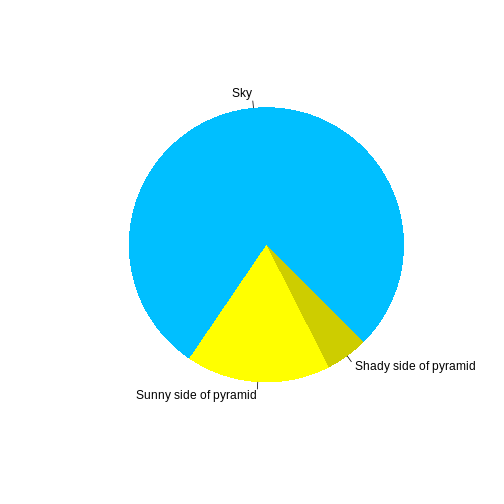
Figures
You can also include figures generated from R Markdown:
R
pie(
  c(Sky = 78, "Sunny side of pyramid" = 17, "Shady side of pyramid" = 5),
  init.angle = 315,
  col = c("deepskyblue", "yellow", "yellow3"),
  border = FALSE
)
Or you can use standard markdown for static figures with the following syntax:
{alt='alt text for accessibility purposes'}
Callout sections can highlight information.
They are sometimes used to emphasise particularly important points but are also used in some lessons to present “asides”: content that is not central to the narrative of the lesson, e.g. by providing the answer to a commonly-asked question.
Math
One of our episodes contains \(\LaTeX\) equations when describing how to create dynamic reports with {knitr}, so we now use mathjax to describe this:
$\alpha = \dfrac{1}{(1 - \beta)^2}$ becomes: \(\alpha = \dfrac{1}{(1 - \beta)^2}\)
Cool, right?
- Use
.mdfiles for episodes when you want static content - Use
.Rmdfiles for episodes when you need to generate output - Run
sandpaper::check_lesson()to identify any issues with your lesson - Run
sandpaper::build_lesson()to preview your lesson locally
Content from Define terms and familiarize with the data
Last updated on 2025-11-11 | Edit this page
Overview
Questions
- What can you expect from this training?
- Where are these data coming from?
- What is a timeseries and why are they important?
Objectives
- Create an R project with folders
- Get familiar with datasets
- Define common terms used to describe timeseries
- Import csv data into R
- Understand differences between base R and tidyverse approaches
About this Lesson
During this lesson we will familiarize ourselves with the data. This data was collected as a part of an NSF funded project, the Aquatic Intermittency effect of Microbiomes in Streams (AIMS; OSF OIA 2019603).
In this episode we will review how to
- Make a project in R
- Familiarize ourselves with the data
- Define common terms used in this lesson
- Import .csv files
- Introuduce differences between coding in base R and using tidyverse.
Getting Started
Before we get familiar with the data, let’s first make sure we remember how to create an R Project, which will help tell our computers where the data exist. The ‘Projects’ interface in RStudio creates a working directory for you and sets the working directory to the project.
Challenge
Using file explorer, create a new folder and R project for this lesson.
What folders would be good to include?
- under the ‘File” menu in RStudio, click on ’New Project’, choose ‘New Directory’, then ‘New Project’
- enter a name for this new directory and where it will be located. This creates your working directory (example: C:/XXX/User/Desktop/Timeseries_R)
- click ‘Create Project’
Creating a timeseries
Start by opening up a new script file in RStudio.
The ‘ts()’ function convertes a numeric vector into a time series R object: ts(vector, start = , end = , frequency = ).
To create a random vector, use ‘sample()’
R
vector <- sample(x = 1:20, size = 50, replace = TRUE)

# x is a vector of the values to sample from (in this example, any number from 1 to 20)
# size is the length of the vector (in this example, 50 characters long)
# replace = TRUE allows values to be repeated in the vector

# To make this vector into a time series, use 'ts()'

timeseries <- ts(vector, start = c(2010, 1), end = c(2015, 12), frequency = 12)
start is the time of first observation (in this example, January 2010) end is the time of final observation (in this example, December 2015) frequency is the number of observations per unit time (1 = annual, 4 = quartly, 12 = monthly)
Exercise #1
Make a basic plot of this timeseries.
R
plot(timeseries)
These plots will look differently for everyone, as we took a random sample to create our vector.
Exercise #2
Using the vector we created, make a timeseries that has annual samples from March 1992 to March 2024 and plot it.
R
annual_ts <- ts(vector, start = c(1992, 3), end = c(2024, 3), frequency = 1)

plot(annual_ts)
Another helpful function for time series is ‘stl()’. This function will decompose the timeseries dataset to identify patterns.
Decomposition is a process that breaks down a time series dataset into different componsents to identify patterns and variations. This helps with predicting (or forecasting) future data points, finding trends, and identifying anomalies in the data (outliers).
Trends in time series occur when there is an overall direction of the data. For example, when the data is increasing, decreasing, or remains constant over time. Outliers are single data points that go far outside the average value of a group of statistics.
In addition to trends, time series data may have other qualities: Seasonality: A regularly repeating pattern of highs and lows related to regular calendar periods such as seasons, quarters, months, or days of the week Cycles: A series of fluctuations that occur over a long period of time, usually multiple years or decades Variation: A change or difference in condition, amount, or level. Often separated into short or long term variation. Stationarity: A times series is considered to be stationarity when the statistical properties do not depend on a time at which the series is observed (there is no temporal trend in the data)
Some other terms to be aware of when working with time series: Missing values: Instances where a value for a specific variable is not recorded or available for a particular observation in a dataset (often recorded as NA or N/A or blank cells)
To look for seasonal decomposition, we can use
R
fit <- stl(timeseries, s.window = "period")

plot(fit)
This function smooths out the seasonal trends in the data, taking the mean and smoothing out remainders to get overall trends in the data.
Understanding the Data
Make sure the data downloaded for surface water and ground water are moved into the ‘data’ folder so you can easily find it.
An important first step for any project is making sure you are familiar with the data.
This lesson uses data collected for the Aquatic Intermittency effects on Microbiomes in Streams (AIMS; NSF OIA 2019603). This project seeks to explore the impacts of stream drying on downstream water quality across Kansas, Oklahoma, Alabama, Idaho, and Mississippi. AIMS integrates datasets on hydrology, microbiomes, macroinvertebrates, and biogeochemistry in three regions (Mountain West, Great Plains, and Southeast Forests) to test the overarching hypothesis that physical drivers (e.g., climate, hydrology) interact with biological drivers (e.g., microbes, biogeochemistry) to control water quality in non-perennial streams. Click here for an overview of the AIMS project.
For our purposes, Non-perennial streams are rivers and streams that cease to flow at some point in time or space and are also commonly referred to as intermittent rivers and ephemeral streams (IRES).
This dataset was collected from an EXO2 Multiparameter Sonde that can measure mutliple water chemistry parameters, including: conductivity, temperature, dissolved oxygen, pH, and others.
One of these sensors was deployed in King’s Creek and the Konza Prairie Biological Station (KPBS).
KPBS is a well known stream study site - famous for its prescirbed
burns and bison grazing. 
Exercise #3
Can you find the Konza Prairie Biological Station on Google Maps? What state did this project take place in? What is the closest city?
This project took place in Kansas, USA. The exact coordinates for this site are: 39°05’32.2”N 96°35’13.9”W
The closest major city is Manhattan, KS.
In this lesson, we will explore the data collected by the sensor at the outlet of the King’s Creek watershed. We will compare groundwater data to surfacewater data to see when the stream dries.
A watershed is an area of land that separates water flowing to different rivers, basins, lakes, or the sea. Groundwater is freshwater that is stored in and orginiates from the ground between soil and rocks. Surfacewater is freshwater found on top fo land in a lake, river, stream, or pond.
Before we load the .csv files into R, try opening them using Excel. Since this will be your first time using the data, it is always a good idea to get familiar with the dataset.
Breakout rooms / At your table, answer the following questions:
Can you see how many time points there are? - When was the first time point? - When was the last time point?
What is the time interval of data collection?
Do you have guesses as to what the columns mean?
Now that we have a better understanding of the data that we will be working with, let’s get started working in R!
Exercise #4
How do you upload a .csv file into R?
R
konza_sw <- read.csv("C://Users/mhope/Desktop/AIMS_GitHub/Carpentries_time_series/data/KNZ_SW_temp_stage_pipeline_mk.csv", header = TRUE)

konza_gw <- read.csv("C://Users/mhope/Desktop/AIMS_GitHub/Carpentries_time_series/data/KNZ_GW_temp_stage_pipeline_mk.csv", header = TRUE)
Once your data is uploaded to R, it can be a lot easier to understand the data.
To get a data summary, use
R
summary(konza_sw)
summary(konza_gw)
Which will tell you the min, 1st quartile, median, mean, 3rd quartile, and maximum values for numeric columns in the dataset.
Many of these numbers will be used to make boxplots of the data:
Boxplot: A method for demonstrating the spread and skewness of the data. Uses min, 1st quartile, median, 3rd quartile, and maximum values
Quartiles: The Q1 (1st Qu.) is the 25% of the data below that point, Q2 is the end of the second quartile and 50th percentile (median), Q3 is the third quartile and is the 75th percentile and upper 25% of the data (3rd. Qu.)
Median: The middle number in an organized list of numbers
Minimum: The lowest number in a list of numbers
Maximum: The highest number in a list of numbers
Another common statistic used is the mean:
Mean: The average of a set of data
Now that we better understand the data, let’s get started on working on cleaning and manipulating the data!
Content from Clean data collected from the field
Last updated on 2025-11-11 | Edit this page
Overview
Questions
- How can you clean time series datasets collected from the field?
Objectives
- Subset rows and columns
- Identify outliers and interpolate missing data
- Filter outliers and missing data
- Create a new dataframe
Introduction
In this episode, we will clean the field data and prepare the data for analysis and visualization. To do this, we will:
- Identify potentially problematic data points (outliers)
- Interpolate missing data
- Change data from UTC to CT
We will use the files Konza_GW.csv and Konza_SW.csv imported in the introduction to the timeseries lesson and the same R packages. Please remember, that we looked at a summary of the data and noticed some weird values. As a reminder we will need packages ggplot2, tidyverse, readr, lubridate, and zoo.
R
install.packages("ggplot2", "tidyverse", "readr", "lubridate", "zoo")

library(ggplot2)
library(tidyverse)
library(readr)
library(lubridate)
library(zoo)
Check the data format
Let’s look at the data structure and make sure the data is in the correct format.
R
str(konza_sw)

# Since my timestamp was imported in as a character I will change the timestamp to a datetime format.
# We can assume the timezones were imported the same way for both datasets.
# The data is in the UTC timezone.

konza_sw$timestamp<- as.POSIXct(konza_sw$timestamp, format = "%m/%d/%Y %H:%M", tz='UTC')
konza_gw$timestamp<- as.POSIXct(konza_gw$timestamp, format = "%m/%d/%Y %H:%M", tz='UTC')

str(konza_sw)
OUTPUT
spc_tbl_ [67,804 × 5] (S3: spec_tbl_df/tbl_df/tbl/data.frame)
$ ...1        : num [1:67804] 1 2 3 4 5 6 7 8 9 10 ...
$ timestamp   : chr [1:67804] "6/9/2021 15:10" "6/9/2021 15:20" "6/9/2021 15:30" "6/9/2021 15:50" ...
$ SW_Temp_PT_C: num [1:67804] -9999 -9999 -9999 -9999 -9999 ...
$ yearMonth   : chr [1:67804] "2021-06" "2021-06" "2021-06" "2021-06" ...
$ SW_Level_ft : num [1:67804] -9999 -9999 -9999 -9999 -9999 ...
- attr(*, "spec")=
 .. cols(
 ..   ...1 = col_double(),
 ..   timestamp = col_character(),
 ..   SW_Temp_PT_C = col_double(),
 ..   yearMonth = col_character(),
 ..   SW_Level_ft = col_double()
 .. )
- attr(*, "problems")=<externalptr>

#after changing to a datetime format
spc_tbl_ [67,804 × 5] (S3: spec_tbl_df/tbl_df/tbl/data.frame)
$ ...1        : num [1:67804] 1 2 3 4 5 6 7 8 9 10 ...
$ timestamp   : POSIXct[1:67804], format: "2021-06-09 15:10:00" "2021-06-09 15:20:00" "2021-06-09 15:30:00" "2021-06-09 15:50:00" ...
$ SW_Temp_PT_C: num [1:67804] -9999 -9999 -9999 -9999 -9999 ...
$ yearMonth   : chr [1:67804] "2021-06" "2021-06" "2021-06" "2021-06" ...
$ SW_Level_ft : num [1:67804] -9999 -9999 -9999 -9999 -9999 ...
- attr(*, "spec")=
 .. cols(
 ..   ...1 = col_double(),
 ..   timestamp = col_character(),
 ..   SW_Temp_PT_C = col_double(),
 ..   yearMonth = col_character(),
 ..   SW_Level_ft = col_double()
 .. )
- attr(*, "problems")=<externalptr>
Since the data is in UTC, we can change the data to Central Time
R
#confirm the data is in UTC

head(konza_sw$timestamp)

#Change the timezone to CT
konza_sw$timestamp<- as.POSIXct(konza_sw$timestamp, format="%Y-%m-%d %H:%M", tz='America/Chicago')
konza_gw$timestamp<- as.POSIXct(konza_gw$timestamp, format="%Y-%m-%d %H:%M", tz='America/Chicago')

#check what timezone our data is in now
head(konza_sw$timestamp)
head(konza_gw$timestamp)
OUTPUT
[1] "2021-06-09 15:10:00 UTC" "2021-06-09 15:20:00 UTC" "2021-06-09 15:30:00 UTC"
[4] "2021-06-09 15:50:00 UTC" "2021-06-09 16:00:00 UTC" "2021-06-09 16:10:00 UTC"

[1] "2021-06-09 10:10:00 CDT" "2021-06-09 10:20:00 CDT" "2021-06-09 10:30:00 CDT" "2021-06-09 10:50:00 CDT"
[5] "2021-06-09 11:00:00 CDT" "2021-06-09 11:10:00 CDT"

[1] "2021-06-09 10:10:00 CDT" "2021-06-09 10:20:00 CDT" "2021-06-09 10:30:00 CDT" "2021-06-09 10:50:00 CDT"
[5] "2021-06-09 11:00:00 CDT" "2021-06-09 11:10:00 CDT"
Plot the data
Now, let’s plot the surface water level data and the water temperature data and evaluate where there might be erroneous values
R
ggplot(data= konza_sw)+                        # name the dataframe you want to use
 geom_line(aes(x=timestamp, y=SW_Level_ft))+   # set the x and y axes
 xlab("Time")+                                 # make a label for the x axis
 ylab("Surface Water Level (ft)")              # make a label for the y axis

Let’s plot the surface water temperature data.
R
ggplot(data= konza_sw)+
 geom_line(aes(x=timestamp, y=SW_Temp_PT_C))+
 xlab("Time")+
 ylab("Temperature (°C)")

Exercise 1: Plot the groundwater dataset and identify outliers.
Fill in the blank: Using code from plotting above to recreate the water level and temperature plots using the groundwater dataset. Visually identify outliers.


Prompt for the learners to discuss.
Looks like we have outliers in our datasets. It is a good idea to zoom in on the outliers and see if there is something weird happening at that time. We can do this by subsetting our data.
Exercise 2: Which piece of code would you use to subset the outliers? Which piece of code would you use to subset NA values? Use this code to change outliers to NA.
Test the following code using the surface water dataset followed by the groundwater dataset. Don’t forget to change the dataframe when evaluating the groundwater dataset:
R
a) konza_sw[c(67780:67830),]
b) konza_sw[konza_sw$timestamp > "2022-09-23 11:50" & konza_sw$timestamp< "2022-09-25 12:00",]
c) subset(konza_sw, SW_Level_ft < 0 )
d) konza_sw[is.na(konza_sw$SW_Level_ft),]

# you can also use the tidyverse package to subset data:

e) konza_sw %>%
  filter(SW_Level_ft < 0)

f) konza_sw %>%
filter(!is.na(SW_Level_ft))OUTPUT
a) # A tibble: 51 × 5
    ...1 timestamp           SW_Temp_PT_C yearMonth SW_Level_ft
   <dbl> <dttm>                     <dbl> <chr>           <dbl>
 1 67780 2022-09-23 14:50:00         19.6 2022-09          0.04
 2 67781 2022-09-23 15:00:00         19.9 2022-09          0.04
 3 67782 2022-09-23 15:10:00         20.4 2022-09      -9999
 4 67783 2022-09-23 15:20:00      -9999   2022-09      -9999
 5 67784 2022-09-23 15:30:00      -9999   2022-09      -9999
 6 67785 2022-09-23 15:40:00      -9999   2022-09      -9999
 7 67786 2022-09-23 15:50:00      -9999   2022-09      -9999
 8 67787 2022-09-23 16:00:00      -9999   2022-09      -9999
 9 67788 2022-09-23 16:10:00      -9999   2022-09      -9999
10 67789 2022-09-23 16:20:00      -9999   2022-09      -9999
# ℹ 41 more rows
# ℹ Use `print(n = ...)` to see more rows

b) # A tibble: 30 × 5
    ...1 timestamp           SW_Temp_PT_C yearMonth SW_Level_ft
   <dbl> <dttm>                     <dbl> <chr>           <dbl>
 1 67775 2022-09-23 14:00:00         18.3 2022-09          0.04
 2 67776 2022-09-23 14:10:00         18.6 2022-09          0.04
 3 67777 2022-09-23 14:20:00         18.9 2022-09          0.04
 4 67778 2022-09-23 14:30:00         19.1 2022-09      -9999
 5 67779 2022-09-23 14:40:00         19.4 2022-09          0.03
 6 67780 2022-09-23 14:50:00         19.6 2022-09          0.04
 7 67781 2022-09-23 15:00:00         19.9 2022-09          0.04
 8 67782 2022-09-23 15:10:00         20.4 2022-09      -9999
 9 67783 2022-09-23 15:20:00      -9999   2022-09      -9999
10 67784 2022-09-23 15:30:00      -9999   2022-09      -9999
# ℹ 20 more rows
# ℹ Use `print(n = ...)` to see more rows

c) # A tibble: 22,000 × 5
    ...1 timestamp           SW_Temp_PT_C yearMonth SW_Level_ft
   <dbl> <dttm>                     <dbl> <chr>           <dbl>
 1     1 2021-06-09 10:10:00      -9999   2021-06         -9999
 2     2 2021-06-09 10:20:00      -9999   2021-06         -9999
 3     3 2021-06-09 10:30:00      -9999   2021-06         -9999
 4     4 2021-06-09 10:50:00      -9999   2021-06         -9999
 5     5 2021-06-09 11:00:00      -9999   2021-06         -9999
 6     6 2021-06-09 11:10:00      -9999   2021-06         -9999
 7     7 2021-06-09 11:20:00      -9999   2021-06         -9999
 8   399 2021-06-12 06:20:00         15.8 2021-06         -9999
 9   442 2021-06-12 13:30:00         18.4 2021-06         -9999
10   443 2021-06-12 13:40:00         18.5 2021-06         -9999
# ℹ 21,990 more rows
# ℹ Use `print(n = ...)` to see more rows


d) # A tibble: 0 × 5
# ℹ 5 variables: ...1 <dbl>, timestamp <dttm>, SW_Temp_PT_C <dbl>, yearMonth <chr>, SW_Level_ft <dbl>

e) 'data.frame':	22000 obs. of  5 variables:
 $ X           : int  1 2 3 4 5 6 7 399 442 443 ...
 $ timestamp   : POSIXct, format: "2021-06-09 10:10:00" "2021-06-09 10:20:00" "2021-06-09 10:30:00" "2021-06-09 10:50:00" ...
 $ SW_Temp_PT_C: num  -9999 -9999 -9999 -9999 -9999 ...
 $ yearMonth   : chr  "2021-06" "2021-06" "2021-06" "2021-06" ...
 $ SW_Level_ft : num  -9999 -9999 -9999 -9999 -9999 ...

f) 'data.frame':	22000 obs. of  5 variables:
 $ X           : int  1 2 3 4 5 6 7 399 442 443 ...
 $ timestamp   : POSIXct, format: "2021-06-09 10:10:00" "2021-06-09 10:20:00" "2021-06-09 10:30:00" "2021-06-09 10:50:00" ...
 $ SW_Temp_PT_C: num  -9999 -9999 -9999 -9999 -9999 ...
 $ yearMonth   : chr  "2021-06" "2021-06" "2021-06" "2021-06" ...
 $ SW_Level_ft : num  -9999 -9999 -9999 -9999 -9999 ...
What did these different methods show? What were the advantages and disadvantages of each method?
Replace bad data values
Now that we know there are numerous weird values, we want to remove those from our dataset by setting them to NA. For surface water level we will remove values below 0 but for temperatures, we will set a low threshold where we will assume the value is incorrect.
R
# base R
konza_sw$SW_Level_ft[konza_sw$SW_Level_ft< 0]<- NA
konza_sw$SW_Temp_PT_C[konza_sw$SW_Temp_PT_C< -100]<- NA

konza_gw$GW_Level_ft[konza_gw$GW_Level_ft< 0]<- NA
konza_gw$GW_Temp_PT_C[konza_gw$GW_Temp_PT_C< -100]<- NA

# tidyR example
konza_sw <- konza_sw %>%
  mutate(SW_Level_ft = replace(SW_Level_ft, SW_Level_ft < 0, NA),
          SW_Temp_PT_C = replace(SW_Temp_PT_C, SW_Temp_PT_C < -100, NA))

konza_gw <- konza_gw %>%
  mutate(GW_Level_ft = replace(GW_Level_ft, GW_Level_ft < 0, NA),
         GW_Temp_PT_C = replace(GW_Temp_PT_C, GW_Temp_PT_C < -100, NA))

#subset and plot to see if our changes worked
subset(konza_sw, SW_Level_ft < 0 )

#plot each dataset and see if it looks ok
ggplot(data= konza_sw)+
  geom_line(aes(x=timestamp, y=SW_Level_ft))+
  xlab("Time")+
  ylab("Surface Water Level (ft)")

ggplot(data= konza_sw)+
  geom_line(aes(x=timestamp, y=SW_Temp_PT_C))+
  xlab("Time")+
  ylab("Temperature (°C)")


ggplot(data= konza_gw)+
  geom_line(aes(x=timestamp, y=GW_Level_ft))+
  xlab("Time")+
  ylab("Surface Water Level (ft)")


ggplot(data= konza_gw)+
  geom_line(aes(x=timestamp, y=GW_Temp_PT_C))+
  xlab("Time")+
  ylab("Temperature (°C)")


Now that we removed bad data values we can count how many NA values are in our dataset. This information may be useful if you need to report your results.
R
#count NA values
sum(is.na(konza_sw$SW_Temp_PT_C))
sum(is.na(konza_sw$SW_Level_ft))
sum(is.na(konza_gw$GW_Temp_PT_C))
sum(is.na(konza_gw$GW_Level_ft))

#divide the number of NA values by the number of rows to see what fraction of our data is NA
sum(is.na(konza_sw$SW_Temp_PT_C)) / nrow(konza_sw)
sum(is.na(konza_sw$SW_Level_ft)) / nrow(konza_sw)
sum(is.na(konza_gw$GW_Temp_PT_C)) / nrow(konza_gw)
sum(is.na(konza_gw$GW_Level_ft)) /nrow(konza_gw)
OUTPUT
[1] 29
[1] 22000
[1] 30
[1] 1884

#divide the number of NA values by the number of rows to see what fraction of our data is NA
[1] 0.0004277034
[1] 0.3244646
[1] 0.0004424518
[1] 0.02778597
Some of these NA values were short intervals that we can interpolate. Let’s interpolate missing values in sections that have less than 12 consecutive NA values and save the interpolated data as a separate column.
R
#interpolate missing values
konza_sw$SW_TEMP_PT_C_int <- na.approx(konza_sw$SW_Temp_PT_C, maxgap = 12, na.rm=FALSE)
konza_sw$SW_Level_ft_int <- na.approx(konza_sw$SW_Level_ft , maxgap = 12, na.rm=FALSE)
konza_gw$GW_TEMP_PT_C_int <- na.approx(konza_gw$GW_Temp_PT_C, maxgap = 12, na.rm=FALSE)
konza_gw$GW_Level_ft_int <- na.approx(konza_gw$GW_Level_ft, maxgap = 12, na.rm=FALSE)
OUTPUT
Exercise 3: Find the new fraction of NA values in the datasets
Adjust the following code for each column and dataset to find the new fraction of NA values:
R
#SW temperature
sum(is.na(konza_sw$SW_TEMP_PT_C_int)) / nrow(konza_sw)

#SW level

#GW temperature

#GW level
OUTPUT
sum(is.na(konza_sw$SW_TEMP_PT_C_int)) / nrow(konza_sw)
[1] 0.0004277034

sum(is.na(konza_sw$SW_Level_ft_int)) / nrow(konza_sw)
[1] 0.3133296

sum(is.na(konza_gw$GW_TEMP_PT_C_int)) / nrow(konza_gw)
[1] 0.004277034

sum(is.na(konza_gw$GW_Level_ft)) /nrow(konza_gw)
[1] 0.02778597
Content from Manipulating a time series data frame
Last updated on 2025-11-11 | Edit this page
Overview
Questions
- How can we reformat our data for analysis and visualization?
- How do we manipulate tabular data in R?
- How and when is it useful to break down a timeseries?
Objectives
- Manipulate a timeseries into different formats for analyses.
- Pivot data from long to wide formats.
- Merge datasets with similar time points.
- Create plots of timeseries data at different temporal scales.
Introduction
In this episode, we will manipulate our cleaned field data for analysis and practice some basic visualization. To do this, we will:
- Change the format of the dataset from “wide” to “long” and back again.
- Combine datasets.
- Create basic plots to observe trends over various time frames.
We will use the files konza_gw.csv and konza_sw.csv cleaned in the previous lession and the same R packages. Please remember, we created new datasets without oultiers or missing datapoints to create a clean dataframe. We will need packages ggplot2, data.table, tidyr, readr, lubridate, zoo, and dplyr.
Depending on your project and the anlyses you want to do, you may want to change the layout of a data set.
Currently, our surface and ground water data sets are in the long format:
R
str(konza_sw)
OUTPUT
data.frame':	67804 obs. of  7 variables:
 $ X               : int  1 2 3 4 5 6 7 8 9 10 ...
 $ timestamp       : POSIXct, format: "2021-06-09 10:10:00" "2021-06-09 10:20:00" "2021-06-09 10:30:00" "2021-06-09 10:50:00" ...
 $ SW_Temp_PT_C    : num  NA NA NA NA NA ...
 $ yearMonth       : chr  "2021-06" "2021-06" "2021-06" "2021-06" ...
 $ SW_Level_ft     : num  NA NA NA NA NA NA NA 1.17 1.16 1.16 ...
 $ SW_TEMP_PT_C_int: num  NA NA NA NA NA ...
 $ SW_Level_ft_int : num  NA NA NA NA NA NA NA 1.17 1.16 1.16 ...
Let’s say we wanted to make the surface water data set into monthly averages, then into long format for plotting in ggplot facets. 1) Using the yearMonth column we will average the temperature and water level data by each year-month 2) melt the data into a long column 3) plot using ggplot
R
#first, lets aggregate the data to yearMonth. We will use our interpolated data columns from the  clean data lesson.
konza_sw_yrmnth<- aggregate(konza_sw[,c(6,7)], list(konza_sw$yearMonth), FUN=mean, na.rm=T) #aggregate the data columns temperature and water level by yearMonth

# tidyr example with group_by() and summarize():
td_sw_yrmth <- tidy_konza_sw %>%
  group_by(yearMonth) %>%
  summarize(SW_TEMP_PT_C_int = mean(SW_TEMP_PT_C_int), na.rm = TRUE,
            SW_Level_ft_int = mean(SW_Level_ft_int), na.rm = TRUE)

#melt the dataframe so that there are three columns; timestamp, value, and variable columns. Note that this uses the data.table melt function.
konza_sw_yrmnth_long<- melt(konza_sw_yrmnth, id.var="Group.1")
konza_sw_yrmnth_long$Group.1<- ym(konza_sw_yrmnth_long$Group.1) #change the character year-month format to a date format. This will add the first day of the month, but we need a day value to format the date value and plot
head(konza_sw_yrmnth_long)

# tidyr example with pivot_longer()
konza_sw_yrmnth_long <- td_sw_yrmth %>%
  pivot_longer(cols = c("SW_TEMP_PT_C_int", "SW_Level_ft_int"),
               names_to = "variable",
               values_to = "value")

#plot the data using ggplot facets
ggplot(data=konza_sw_yrmnth_long)+
  geom_line(aes(x=Group.1, y=value))+
  geom_point(aes(x=Group.1, y=value))+
  facet_grid(variable~., scales='free',
             labeller=as_labeller(c('SW_TEMP_PT_C_int'='Surface Water Temperature (°C)','SW_Level_ft_int'= "Surface Water Level (ft)")))+
  theme_bw()

# for the tidyr example, Group.1 = yearMonth
OUTPUT
#The aggregated konza sw data should look like the dataframe below
Group.1 SW_TEMP_PT_C_int SW_Level_ft_int
1  2021-06               NA              NA
2  2021-07      17.18803987       0.8641611
3  2021-08      24.95998656              NA
4  2021-09      20.27976820              NA
5  2021-10      14.24646306              NA
6  2021-11       9.85321991              NA
7  2021-12       5.54276295              NA
8  2022-01      -1.83456541              NA
9  2022-02      -0.01608879              NA
10 2022-03       6.81216816              NA
11 2022-04      11.85371296       1.1746100
12 2022-05      14.92028002       1.2461929
13 2022-06      17.90387561       1.3941239
14 2022-07      17.15921991       1.3757745
15 2022-08      21.30550236              NA
16 2022-09               NA              NA

      Group.1         variable    value
1 2021-06-01 SW_TEMP_PT_C_int 15.50090
2 2021-07-01 SW_TEMP_PT_C_int 17.18804
3 2021-08-01 SW_TEMP_PT_C_int 24.95999
4 2021-09-01 SW_TEMP_PT_C_int 20.27977
5 2021-10-01 SW_TEMP_PT_C_int 14.24646
6 2021-11-01 SW_TEMP_PT_C_int  9.85322
Let’s say we wanted to make the surface water data set into an annual timeframe. To do this we will: - add a column that only includes the year - aggregate our data by the year column
R
#add the year column
konza_sw$yr<- year(konza_sw$timestamp)
head(konza_sw)

# using tidyr; mutate()
konza_sw <- konza_sw %>%
  mutate(yr = year(konza_sw$timestamp))

#aggregate by year
konza_sw_annual<- aggregate(konza_sw[,c(6,7)], list(konza_sw$yr), FUN=mean, na.rm=T)
head(konza_sw_annual)

# using tidyr; summarize()
konza_sw_annual <- konza_sw %>%
  group_by(yr) %>%
  summarize(SW_TEMP_PT_C_int = mean(SW_TEMP_PT_C_int, na.rm = TRUE),
            SW_Level_ft_int = mean(SW_Level_ft_int, na.rm = TRUE))
OUTPUT
# A tibble: 6 × 8
   ...1 timestamp           SW_Temp_PT_C yearMonth SW_Level_ft SW_TEMP_PT_C_int SW_Level_ft_int    yr
  <dbl> <dttm>                     <dbl> <chr>           <dbl>            <dbl>           <dbl> <dbl>
1     1 2021-06-09 10:10:00           NA 2021-06            NA               NA              NA  2021
2     2 2021-06-09 10:20:00           NA 2021-06            NA               NA              NA  2021
3     3 2021-06-09 10:30:00           NA 2021-06            NA               NA              NA  2021
4     4 2021-06-09 10:50:00           NA 2021-06            NA               NA              NA  2021
5     5 2021-06-09 11:00:00           NA 2021-06            NA               NA              NA  2021
6     6 2021-06-09 11:10:00           NA 2021-06            NA               NA              NA  2021


Group.1 SW_TEMP_PT_C_int SW_Level_ft_int
1    2021         15.34314       0.5591678
2    2022         12.01738       1.0039842
Change the groundwater data frame into a yearMonth dataframe and an annual dataframe
Fill in the blank in the code below to aggregate the data by year-month, melt to long format, and aggregate the data by year for the groundwater data
R
#aggregate to year-month
konza_gw_yrmnth<- aggregate(_______, list(___________), FUN=mean, na.rm=T)

# using tidyR to summarize()
konza_gw_yrmnth <- konza_gw %>%
  group_by(_____) %>%
  summarize(SW_TEMP_PT_C_int = _____(SW_TEMP_PT_C_int, na.rm = ____),
            SW_Level_ft_int = _____(SW_Level_ft_int, na.rm = ____))


#melt the dataframe so that there are three columns
konza_gw_yrmnth_long<- melt(_____, id.var="Group.1")
konza_gw_yrmnth_long$Group.1<- ym(konza_gw_yrmnth_long$Group.1) #change the character year-month format to a date format
head(konza_gw_yrmnth_long)

# using tidyr
konza_gw_yrmnth_long <- konza_gw_yrmnth %>%
  pivot_longer(cols = c("_______", "_______"),
               names_to = "_______",
               values_to = "______")

#add the year column
konza_gw$yr<- year(________)
head(konza_sw)

# use mutate to add 'yr' column
konza_gw <- konza_gw %>%
  ______(yr = year(konza_gw$_____))
head(konza_gw)


#aggregate by year
konza_gw_annual<- aggregate(________, list(_________), FUN=mean, na.rm=T)
head(konza_gw_annual)

# summarize by year
konza_gw_annual <- konza_gw %>%
  group_by(_____) %>%
  summarize(SW_TEMP_PT_C_int = _____(SW_TEMP_PT_C_int, na.rm = TRUE),
            SW_Level_ft_int = ______(SW_Level_ft_int, na.rm = TRUE))

#format the date column
konza_gw_yrmnth_long$Group.1<- ym(__________)OUTPUT
#aggregate to year-month
konza_gw_yrmnth<- aggregate(konza_gw[,c(10,11)], list(konza_gw$yearMonth), FUN=mean, na.rm=T)

#melt the dataframe so that there are three columns
konza_gw_yrmnth_long<- melt(konza_gw_yrmnth, id.var="Group.1")
konza_gw_yrmnth_long$Group.1<- ym(konza_gw_yrmnth_long$Group.1) #change the character year-month format to a date format
head(konza_gw_yrmnth_long)

     Group.1         variable    value
1 2021-06-01 GW_TEMP_PT_C_int 13.96984
2 2021-07-01 GW_TEMP_PT_C_int 15.80226
3 2021-08-01 GW_TEMP_PT_C_int 19.76004
4 2021-09-01 GW_TEMP_PT_C_int 19.54039
5 2021-10-01 GW_TEMP_PT_C_int 16.45497
6 2021-11-01 GW_TEMP_PT_C_int 12.07231

#add the year column
konza_gw$yr<- year(konza_gw$timestamp)
head(konza_sw)

# A tibble: 6 × 8
   ...1 timestamp           SW_Temp_PT_C yearMonth SW_Level_ft SW_TEMP_PT_C_int SW_Level_ft_int    yr
  <dbl> <dttm>                     <dbl> <chr>           <dbl>            <dbl>           <dbl> <dbl>
1     1 2021-06-09 10:10:00           NA 2021-06            NA               NA              NA  2021
2     2 2021-06-09 10:20:00           NA 2021-06            NA               NA              NA  2021
3     3 2021-06-09 10:30:00           NA 2021-06            NA               NA              NA  2021
4     4 2021-06-09 10:50:00           NA 2021-06            NA               NA              NA  2021
5     5 2021-06-09 11:00:00           NA 2021-06            NA               NA              NA  2021
6     6 2021-06-09 11:10:00           NA 2021-06            NA               NA              NA  2021

#aggregate by year
konza_gw_annual<- aggregate(konza_gw[,c(10,11)], list(konza_gw$yr), FUN=mean, na.rm=T)
head(konza_gw_annual)

  Group.1 GW_TEMP_PT_C_int GW_Level_ft_int
1    2021          15.2877        2.420264
2    2022          12.4111        2.461994
Compare groundwater and surface water data
What if we want to compare the monthly surface water and groundwater values? We can merge the two dataframes and plot both together. Note - to merge the datasets by adding rows using rbind() below, both datasets need the exact same columns
Add a dataset column, and bind the month-day groundwater and surface water dataframes
R
#add the datasets so we can keep track of which data belongs where
konza_gw_yrmnth_long$dataset<- 'Groundwater'
konza_sw_yrmnth_long$dataset<- 'Surface Water'

# you can also do this with mutate
konza_gw_yrmnth_long <- konza_gw_yrmnth_long %>%
  mutate(dataset = 'Groundwater')
konza_sw_yrmnth_long <- konza_sw_yrmnth_long %>%
  mutate(dataset = 'Surface Water')

#since the columns are the same, we can use rbind to combine the dataframes
# rbind is "row bind" - only possible when the two datasets have the same columns
konza_yrmnth<- rbind(konza_gw_yrmnth_long, konza_sw_yrmnth_long)

#remove GW and SW labels from the variable columns so that we can plot these variables together for groundwater and surface water
konza_yrmonth$variable<- gsub(pattern = 'GW_', replacement = "", konza_yrmonth$variable)
konza_yrmonth$variable<- gsub(pattern = 'SW_', replacement = "", konza_yrmonth$variable)

# can also use mutate() in tidyR
konza_yrmnth <- konza_yrmnth %>%
  mutate(pattern = 'SW_', replacement = "", variable,
         pattern = 'GW_', replacement = "", variable)
OUTPUT
     Group.1      variable    value     dataset
1 2021-06-01 TEMP_PT_C_int 13.96984 Groundwater
2 2021-07-01 TEMP_PT_C_int 15.80226 Groundwater
3 2021-08-01 TEMP_PT_C_int 19.76004 Groundwater
4 2021-09-01 TEMP_PT_C_int 19.54039 Groundwater
5 2021-10-01 TEMP_PT_C_int 16.45497 Groundwater
6 2021-11-01 TEMP_PT_C_int 12.07231 Groundwater
Next, plot the dataframes using ggplot
R
ggplot(data=konza_yrmonth)+
  geom_line(aes(x=Group.1, y=value, color=dataset))+
  geom_point(aes(x=Group.1, y=value, color=dataset))+
  xlab('Date')+
  facet_grid(variable~., scales='free',
             labeller=as_labeller(c('TEMP_PT_C_int'='Water Temperature (°C)',
                                                             'Level_ft_int'= "Water Level (ft)")))+
  theme_bw()

# if using the tidyr examples, Group.1 = yearMonth

Save the cleaned dataframes
We can use R to create versions of our cleaned dataframes so we won’t have to go back and run the code from the previous lesson every time we want to work with the data.
To keep our R project neat, save these files in the folder “data_processed”.
Tip - use names that are short, but clear.
When working in R, sometimes you can have a lot of files open in your environment, making it difficult to keep track of what you are working on.
It can be helpful to periodically remove files to keep a clean environment.
You can do this with individual files using the function rm()
R
rm(konza_sw)
rm(konza_gw)
or by cleaning out the full environment all at once
R
rm(list = ls())
BE AWARE! Whenever you remove something from the environment there is no easy “back” or “undo” button in R. Always make sure you have the version of the files that you need to continue with your work!
In the next episode we will start by uploading our 3 cleaned data frames.